Every Color Space You Edit In Was Defined by the Eyes of 17 People in 1920s England

In a darkened room at Imperial College in London in the late 1920s, ten people looked at a small split circle of light, about the width of a thumbnail held at arm's length. Half the circle carried a single wavelength; the other half carried a mixture of red, green, and blue lamps the subject could turn up and down until the two halves fused into one uniform patch. Seven more people did the same job at the National Physical Laboratory in Teddington, and the numbers those 17 people generated are still sitting inside every ICC profile on your computer.

The chain is short and unbroken. sRGB, Adobe RGB (1998), Display P3, Rec. 2020, and ProPhoto RGB are all defined by naming their red, green, and blue primaries as xy coordinates on the CIE 1931 chromaticity diagram. CIELAB is a transform of CIE XYZ. The delta E numbers your photo and calibration tools report are distances measured in CIELAB. ICC color management runs everything through a profile connection space built on CIE XYZ or CIELAB under illuminant D50 and the CIE 1931 2-degree standard colorimetric observer. Pull the thread on any of it and you arrive at a handful of British lab volunteers turning knobs.

What the 17 Observers Actually Did

The apparatus was a trichromatic colorimeter, and the task was a bipartite field match. The observer saw a circular field split down the middle into two semicircles. One side showed the test light, a narrow band pulled out of a spectrum. The other side showed an additive mixture of three primary lights whose intensities the observer controlled. The job was to make the seam disappear.

W. David Wright ran the Imperial College group with monochromatic primaries at 650, 530, and 460 nm, stepping through the spectrum from 400 to 700 nm at 10 nm intervals. John Guild ran the National Physical Laboratory group with broadband primaries made by putting red, green, and blue gelatin filters in front of an opal-bulb lamp, working from 380 to 700 nm at 5 nm intervals. Two different labs, two different instruments, two different sets of primaries, 17 people between them. Wright's 1929 paper appeared in the Transactions of the Optical Society; Guild's 1931 paper appeared in the Philosophical Transactions of the Royal Society A.

The two datasets were then converted onto a shared set of reference primaries at 700, 546.1, and 435.8 nm, and the results agreed far more closely than two samples that size had any business doing. That agreement is what gave the international committee the nerve to standardize. At its eighth session, held in Cambridge in 1931, the Commission Internationale de l'Éclairage adopted the combined data as the standard colorimetric observer, and the field of colorimetry got its foundation.

Some spectral test lights cannot be matched by any positive mixture of three real primaries; the mixture is always too pale. The fix was to move a primary across the seam and add it to the test side instead, then record its contribution as a negative number. That is why the CIE RGB color-matching function for red dips below zero across much of the blue-green region, and it is why a three-primary display gamut is a triangle sitting inside a horseshoe it can never fill. Add a fourth or fifth primary, as multiprimary LCDs with yellow and cyan channels have done, and the gamut becomes a convex polygon instead, still trapped inside the horseshoe but reaching further into it.

The Part That Was Never Measured

The popular telling is that the standard observer is the average human eye, a careful statistical portrait of normal color vision. It is not that, and the size of the sample behind it was never a secret. It is an average of 17 volunteers drawn from two English physics laboratories, all of them screened as color normal, all of them adults available to sit for long sessions in a dark room in the 1920s. Guild wrote in his own paper that Wright's ten observers agreed with the seven at the National Physical Laboratory more closely than the size of either group should have led anyone to expect, which is a statement about luck as much as about biology.

The sample size is not even the deepest problem. The CIE 1931 color-matching functions were not measured directly at all. Wright and Guild produced relative chromaticity data, which fixes the shape of the color triangle but not the brightness attached to it. To turn that into a full set of color-matching functions, the committee imposed a constraint: the y-bar curve would be forced to equal the 1924 CIE photopic luminous efficiency function, the standard curve for how bright a watt of light looks at each wavelength. The 1931 observer is therefore a reconstruction, built by fitting one lab's chromaticity data to another era's brightness curve. The Colour and Vision Research Laboratory at University College London describes both the borrowed brightness curve and the reconstruction itself as questionable.

The 1924 brightness curve had its own provenance problem. It was assembled from luminosity measurements taken by several groups using several different methods, and it did not come from the 17. So the headline number is right about the chromaticity half of the standard observer and understates the mess in the other half. Seventeen people set the shape. A committee's compromise between separate experiments set the brightness weighting that runs through it.

Why the Blues Were Always the Weak Spot

That borrowed brightness curve is the origin of the best-documented defect in the whole system. The 1924 function seriously underestimates human sensitivity in the violet, and the size of the miss approaches an order of magnitude at the short end. Because y-bar was defined to be that curve, the error was welded directly into the luminance channel of CIE XYZ, and from there into CIELAB lightness, into delta E, and into every profile that uses them.

The color science community has known this since at least 1951, when Deane Judd published a revised luminous efficiency function with corrections confined to wavelengths below 460 nm. J. J. Vos refined Judd's version in 1978. Neither replacement was adopted as the general standard for imaging, partly because Judd's correction carries its own artifact: the modified curve implies a standard observer with an unrealistically high macular pigment density, so it trades one distortion for a smaller one.

For most photography, the practical consequence is modest, because most of what you shoot is broadband and the error lives at the edge of the spectrum. It stops being modest when the light is narrow. Deep blue and violet LEDs, laser projection, saturated blue stage lighting, and the blue primary of a wide gamut display all sit close to the region where the 1931 functions are least trustworthy. If you have ever measured a deep blue and gotten a number that felt wrong compared to what you saw, you were not necessarily imagining it.

The 10-Degree Observer and the Ones After It

The 1931 field was 2 degrees wide, which confines the stimulus to the central fovea, where cone density is highest and rods are scarce. At a normal monitor viewing distance of about 24 inches, 2 degrees covers a patch roughly 0.8 inches across. Almost nothing you actually evaluate on screen is that small. Skin on a full-page portrait, a sky, a wall of product packaging, a print held at reading distance: all of it is a large field, and large fields land on the retina with a different amount of macular pigment in front of them. That yellow screen is dense over the central fovea and thins out beyond it, so a wide field reaches the cones through less of it and matches differently.

The CIE addressed that in 1964 with a supplementary observer built for 10-degree fields, and it addressed it with a much better dataset. Rods do sit out in that wider field, but they are deliberately not part of what the standard describes: the 1964 observer is specified for high photopic levels and for spectral conditions in which no rod participation is expected, and the experimenters worked to suppress rod influence in the matches themselves. W. S. Stiles and J. M. Burch measured 49 observers at the National Physical Laboratory from 392.2 to 714.3 nm, using primaries near 645, 526, and 444 nm, and their color-matching functions were measured directly rather than reconstructed from a borrowed brightness curve. Their final report appeared in 1959, and N. I. Speranskaya published matches from 27 observers the same year. The 1964 observer leans mainly on the Stiles and Burch data, with the Speranskaya set as a secondary contribution, and the CIE adjusted and smoothed both before publishing. The recommendation that came out of it is straightforward: use the 10-degree observer when the color-matching field is bigger than about 4 degrees.

Practically nobody does. Your camera profiles, your display profiles, your printer profiles, your soft proof, and your delta E readout all run on the 2-degree observer from 1931. Whether that is the wrong instrument for a photograph is a harder question than the angles make it look, because the 4-degree rule describes a matching field rather than the width of a picture, and experiments with real images suggest complex scenes behave as though the effective field is smaller than the screen area they cover. The mismatch is real. It is not the tidy 30-degrees-against-2 arithmetic it first appears to be. The CIE has since published cone-fundamental-based functions for both field sizes, in CIE 170-1 in 2006 and CIE 170-2 in 2015, built on cone spectral sensitivities estimated from the Stiles and Burch matches and from observers of known genotype rather than on the 1924 brightness curve. Industry uptake has been close to nil. Writing in LD+A, the journal of the Illuminating Engineering Society, Jess Baker, Tony Esposito, and Jason Livingston attribute the 1931 observer's survival to the inertia that has to be overcome before anyone changes a metric.

Two Honest People, One Calibrated Monitor

None of this means the standard observer is wrong. It means it is a single fixed answer to a question that has a distribution of answers. Human color matching varies between people with entirely normal vision, driven by macular pigment density, by the optical density of cone photopigment, by a common genetic polymorphism in the long-wavelength cone, and by the lens of the eye yellowing steadily with age. Two people can look at the same patch on the same calibrated monitor, see genuinely different colors, and both be describing their own retinas accurately.

Color scientists call this observer metamerism, and it gets worse as primaries get narrower. A display or projector whose red, green, and blue outputs are spectrally narrow spikes will drive a large gamut, and it will also amplify the difference between two observers, because a small shift in where someone's cone sensitivities peak changes how much of a narrow spike they catch. Modeling work using measured individual cone functions has put average observer metamerism indices for laser projection in the range of roughly one to two units of color difference with maxima around three, with near-neutral bright tones among the areas where individuals disagree most. Those are not enormous numbers. They are also comfortably larger than the tolerances people argue about in a color-critical review.

The measuring instruments inherit the same assumption. A display colorimeter such as the Calibrite Display Plus HL reports tristimulus values by approximating the 1931 functions with filters, which is why calibration software ships with correction data per display technology. The puck is not measuring color. It is measuring light and then asking what 17 English volunteers would have said about it.

How to Argue About Color Without Losing

A number in a color-managed pipeline is a prediction about a hypothetical observer, not a description of the person standing behind you. Delta E answers the question of whether two stimuli would have matched for the 1931 average. It does not answer whether they match for your client, and there is no calibration that can make it answer that. As the LD+A authors put it, "It is simply not possible to create a color match for all people simultaneously, even if all viewers have normal color vision."

That has concrete consequences for how you run a review. When a client says the skin has gone green and your numbers say it has not, telling them the numbers win is both rude and, strictly speaking, unjustified. What the numbers establish is that your file will behave predictably as it moves between devices, which is the actual job color management was invented to do. Appearance disputes get settled by putting the disputing parties in front of the same display, in the same room light, at the same distance, looking at the same size patch. Move the argument from the abstract to a shared retinal experience, and most of it evaporates.

Keep the technical conversation and the aesthetic conversation separate, because the first has a right answer and the second does not. Lean on relationships rather than absolutes when you can, because a retoucher who has spent years color grading portraits is reading how a skin tone sits against the background and the wardrobe, and those relationships survive observer differences far better than any single coordinate does.

ProPhoto RGB makes the abstraction impossible to ignore. Two of its three primaries sit outside the spectral locus entirely, which means they correspond to no physical light at all, and a commonly cited figure puts about 13% of the codes in the space on colors no human being can see. Those coordinates exist because a horseshoe drawn from 17 people's knob settings in 1931 is the map, and Kodak's engineers needed corners outside it to enclose the real-world surface colors a photograph has to hold. Even so, the triangle misses part of the horseshoe: saturated blue-greens near 500 nm fall outside it. Every time you open a ProPhoto file, you are working inside a container whose edges were fixed by the limits of what a small group of volunteers in two English laboratories could match with three lamps.

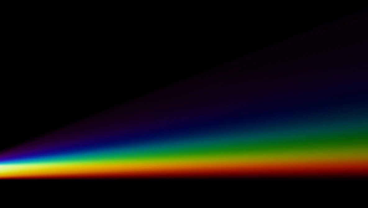
Lead image by Kilohn limahn, CC BY-SA 4.0. Source.